
The Incident
A fraud detection model with 98% test accuracy was silently blocking legitimate customers for six months.
No alerts fired. No system crashed. The dashboards looked healthy.
But the business was losing $765,000 every month.
The model wasn’t broken in development — it was broken in production.
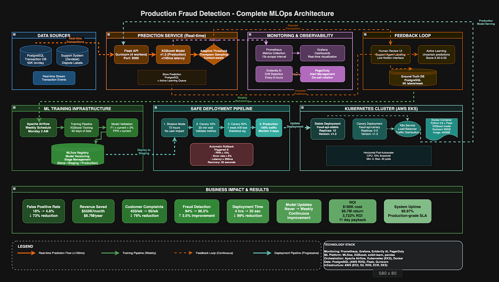
This case study explains how the failure wasn’t caused by bad machine learning, but by missing MLOps practices. Over eight weeks, I redesigned the system into a production ML platform, reducing false positives from 18% to 4.8% and recovering $6.7M annually.
This document covers the technical implementation, architecture decisions, tools selected, and lessons learned for engineers operating machine learning systems in real production environments.
Initial Deployment and Failure Analysis
I was assigned to build a fraud detection system for a payment processing platform handling 50,000 daily transactions. After three months of development, I trained an XGBoost model achieving 98% accuracy on historical test data spanning two years.
The deployment approach I used was straightforward but ultimately flawed. I serialized the trained model to a pickle file, wrote a prediction service in Python, and deployed it to production with a fixed threshold of 0.5. Any transaction scoring above this threshold was automatically blocked.
The deployment included no monitoring infrastructure, no feedback mechanisms, and no versioning system. I operated under the assumption that test set performance would translate directly to production performance.
Six months post-deployment, analysis revealed the model was blocking 18% of legitimate transactions. Customer complaints increased 340%. Revenue loss from false positives totaled $765K monthly. The churn rate increased from 3% to 8%.
Root Cause Analysis
Investigation identified five critical failures in the initial deployment:
- Lack of Production Monitoring
There was no instrumentation to track model performance in production. The false positive rate went undetected for months until business metrics revealed the problem. - Training-Serving Skew
The model was trained on data collected 9–12 months prior. Production data had shifted significantly: average transaction amounts increased 30%, payment method distributions changed with new digital wallet adoption, and geographic patterns shifted as the business expanded. - Static Decision Threshold
The fixed 0.5 threshold applied uniformly across all transaction contexts. A $5 purchase from a three-year customer received identical treatment to a $1000 first-time transaction from a new account. - No Feedback Loop
Customer disputes verified by support agents generated valuable ground truth labels, but this data remained siloed in ticketing systems. The model could not learn from its production mistakes. - Absence of Safe Deployment Practices
The model was deployed directly to 100% of traffic with no validation against production data and no rollback capability.
Solution Architecture: MLOps Implementation
I designed an eight-week implementation plan to address each failure point systematically. The solution required building monitoring infrastructure, feedback collection systems, adaptive decision logic, safe deployment pipelines, and automated retraining.
Phase 1: Production Monitoring Infrastructure (Weeks 1–2)
The first priority was gaining visibility into production model behavior. I selected Prometheus for metrics collection due to its time-series capabilities and ecosystem integration.
Tool Selection: Prometheus
What is Prometheus:
Prometheus is an open-source monitoring and alerting system originally built at SoundCloud. It collects and stores metrics as time-series data, recording information with timestamps. It uses a pull-based model, scraping metrics from instrumented applications at defined intervals.
Why I chose Prometheus:
I evaluated several monitoring solutions including Datadog, New Relic, and CloudWatch. I selected Prometheus for four key reasons:
- Open-source and cost-effective: No per-metric pricing that could scale unpredictably
- Powerful query language (PromQL): Enables complex metric aggregations and analysis
- Built for high-cardinality data: Handles ML model metrics with multiple dimensions effectively
- Strong ecosystem integration: Native support in Kubernetes and integration with Grafana
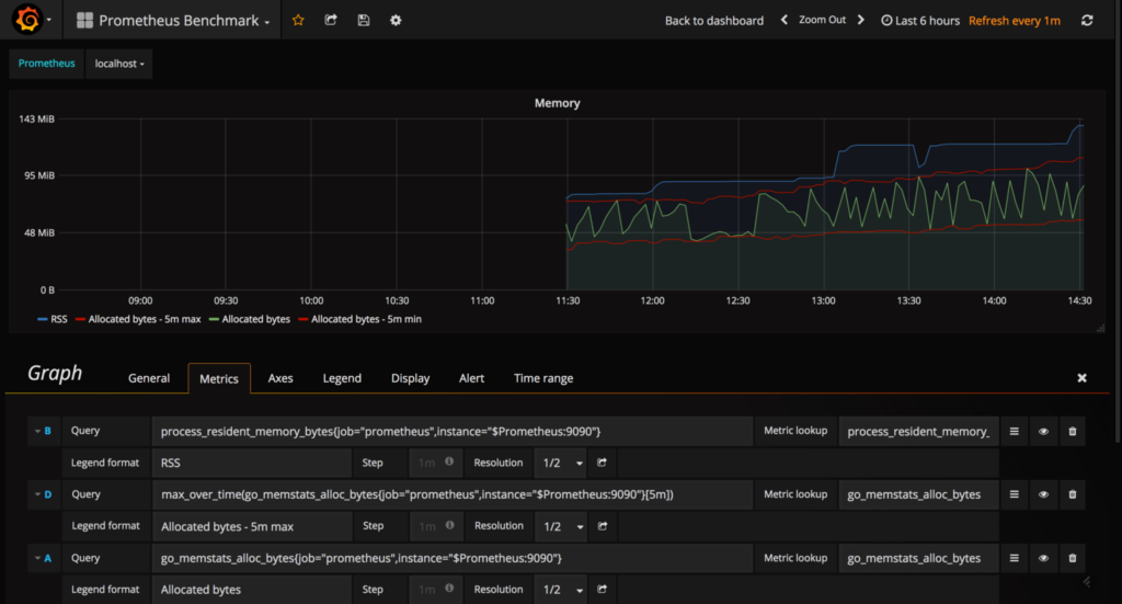
How I used it in this project:
I instrumented my fraud detection service to expose metrics on port 9090. Prometheus scraped these metrics every 15 seconds. I tracked prediction counts, latency distributions, score distributions, and custom business metrics like false positive rate. The time-series data enabled trend analysis to identify gradual performance degradation.
Instrumentation Implementation
from prometheus_client import Counter, Histogram, Gauge
# Define metrics
predictions_total = Counter(
    'fraud_predictions_total',
    'Total predictions by outcome',
    ['model_version', 'outcome']
)
prediction_latency = Histogram(
    'fraud_prediction_latency_seconds',
    'Prediction latency distribution',
    buckets=[0.01, 0.025, 0.05, 0.1, 0.25, 0.5]
)
false_positive_rate = Gauge(
    'fraud_fpr',
    'False positive rate over sliding window'
)
def predict_transaction(features):
    start = time.time()
    score = model.predict_proba([features])[0][1]
    decision = 'block' if score > threshold else 'approve'
    predictions_total.labels(
        model_version=MODEL_VERSION,
        outcome=decision
    ).inc()
    prediction_latency.observe(time.time() - start)
    return {'score': score, 'decision': decision}
Prometheus Configuration
groups:
  - name: fraud_detection
    rules:
      - alert: HighFPR
        expr: fraud_fpr > 0.12
        for: 5m
        annotations:
          summary: "FPR exceeded 12%"
     - alert: CriticalFPR
        expr: fraud_fpr > 0.15
        for: 2m
        annotations:
          summary: "FPR critical - consider rollback"
Tool Selection: Grafana
What is Grafana:
Grafana is an open-source analytics and interactive visualization platform. It connects to data sources like Prometheus and transforms raw metrics into customizable dashboards with graphs, charts, and alerts. It provides a web interface for real-time monitoring.
Why I chose Grafana:
After implementing Prometheus, I needed a visualization layer. I chose Grafana over alternatives like Kibana or custom dashboards because:
- Native Prometheus integration
- Rich visualization options
- Alert integration
- Template variables
- Community dashboards
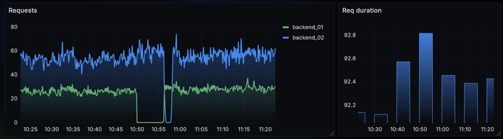
How I used it:
I created three primary dashboards. The executive dashboard displayed high-level business metrics with color-coded thresholds. The engineering dashboard showed technical metrics like latency percentiles and error rates. The drift analysis dashboard visualized feature distribution changes over time. Each dashboard refreshed every 30 seconds and included drill-down capabilities for detailed investigation.
Visualization Implementation
I built Grafana dashboards displaying:
– False positive rate trend with threshold indicators (primary metric)
– Prediction latency at p50, p95, p99 with SLA lines
– Prediction volume and distribution by decision type
– Score distribution histogram comparing current vs historical
– Error rates by error type with automatic annotations
Configuration example for the FPR panel:
{
  "title": "False Positive Rate",
  "targets": [{
    "expr": "fraud_fpr",
    "legendFormat": "FPR"
  }],
  "alert": {
    "conditions": [{
      "evaluator": {"type": "gt", "params": [0.12]}
    }]
  }
}
This monitoring infrastructure provided real-time visibility for the first time since deployment. The dashboards were displayed on monitors in the engineering area and accessible via mobile for on-call engineers.
Tool Selection: Evidently AI
What is Evidently AI:
Evidently is an open-source Python library designed specifically for ML model monitoring. It analyzes data quality, data drift, model performance, and target drift by comparing reference data (training set) against current data (production). It generates interactive HTML reports and JSON outputs for integration with monitoring systems.
Why I chose Evidently AI:
While Prometheus tracks generic application metrics, I needed ML-specific monitoring. I evaluated Evidently AI, Whylabs, and Fiddler. I selected Evidently because:
- ML-focused metrics: Built-in drift detection using statistical tests (Kolmogorov-Smirnov, Population Stability Index)
- Open-source: No vendor lock-in, full control over deployment
- Multiple drift detection methods: Automatically selects appropriate test based on feature type
- Visual reports: HTML reports help explain drift to non-technical stakeholders
- Integration-friendly: JSON output integrates with Prometheus and alerting systems
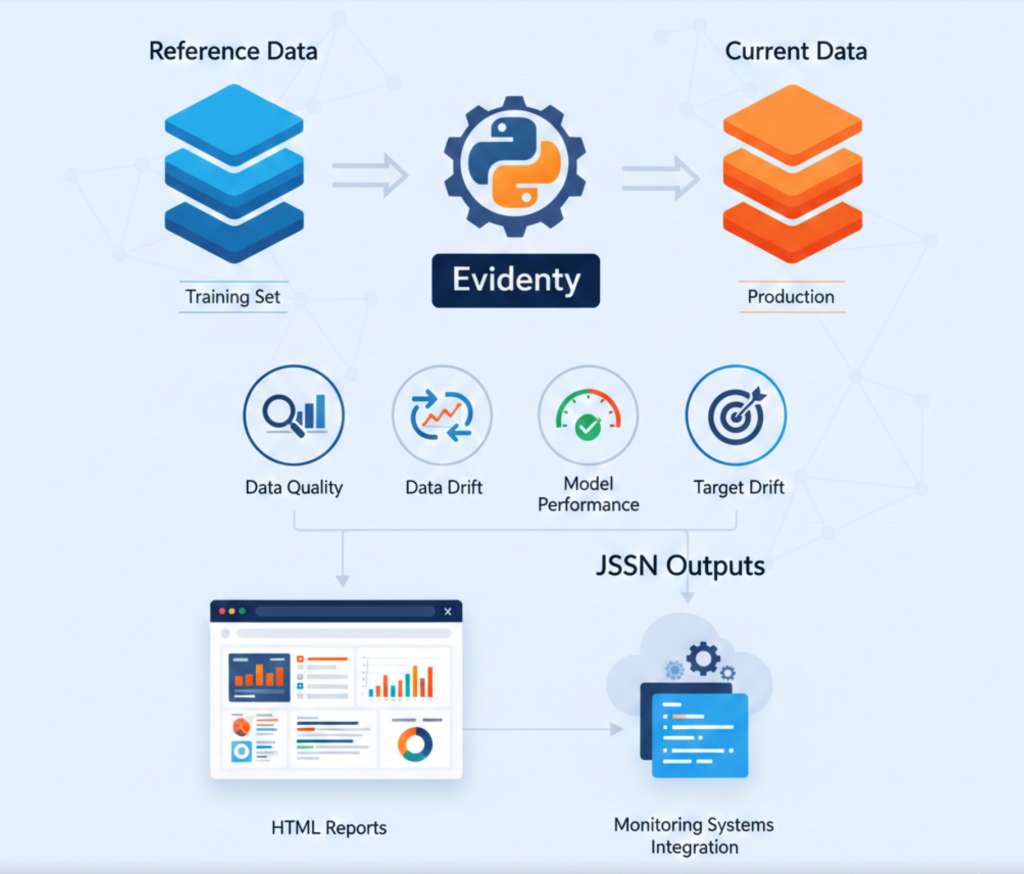
How it was used:
I scheduled Evidently drift checks every 6 hours. The system compared the most recent 10,000 production transactions against the original training dataset. For each feature, Evidently calculated drift scores and determined if distribution shifts were statistically significant. I configured it to send drift scores to Prometheus as custom metrics, enabling Grafana visualization and alerting.
Findings:
Transaction amount drift: 32%
Payment method drift: 45%
Geographic drift: 28%
Phase 2: Feedback Loop Implementation (Weeks 3–4)
The second phase focused on capturing ground truth labels from production to enable model improvement.
Tool Selection: PostgreSQL
What is PostgreSQL:
PostgreSQL is an open-source relational database management system emphasizing extensibility and SQL compliance. It supports complex queries, foreign keys, triggers, and JSONB data type for semi-structured data. It provides ACID transactions and robust data integrity guarantees.
Why I chose PostgreSQL:
I needed a database to store predictions, ground truth labels, and feedback data. I evaluated PostgreSQL, MongoDB, and Snowflake. I selected PostgreSQL because:
- JSONB support: Store variable feature sets without rigid schema while maintaining queryability
- Relational integrity: Foreign keys ensure predictions and labels remain consistent
- Complex query support: Join predictions with ground truth for training data extraction
- Transaction guarantees: ACID properties critical for financial fraud data
- Mature ecosystem: Well-tested with extensive tooling and client libraries
- Cost-effective: Self-hosted without per-query pricing
How it was used:
I deployed PostgreSQL 14 on AWS RDS with automated backups and read replicas. The database stored all predictions with full feature context in JSONB columns. Ground truth labels linked to predictions via foreign keys. I created indexes on timestamp and transaction_id columns for efficient queries. The training pipeline queried this database to extract labeled data for retraining. Total storage grew to approximately 50GB over three months with 4 million prediction records.
Within the first week, this system collected 1,200 new labeled examples. By week four, I had accumulated 5,000 labels. This created a continuously growing training dataset capturing current production patterns.
Phase 3: Adaptive Threshold System (Weeks 4–5)
Analysis showed that applying a single threshold across all transaction contexts was suboptimal. I designed a contextual threshold system using multi-armed bandit optimization.
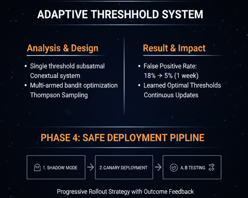
Result:
Deploying adaptive thresholds reduced the false positive rate from 18% to 5% within one week. The system learned optimal threshold application through continuous Thompson Sampling updates based on outcome feedback.
Phase 4: Safe Deployment Pipeline (Weeks 5–6)
To deploy model updates safely, I implemented a progressive rollout strategy with three stages: shadow mode, canary deployment, and A/B testing.
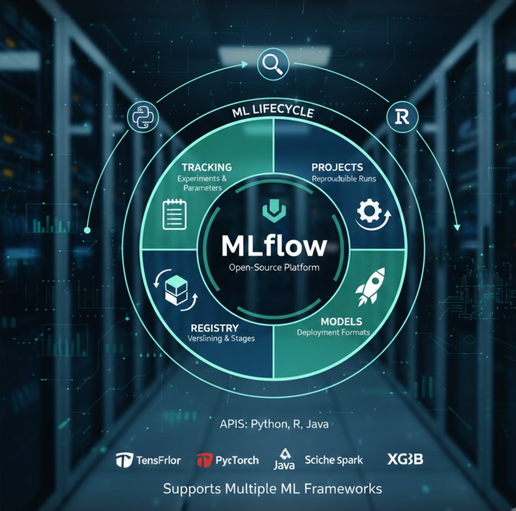
Tool Selection: MLflow
What is MLflow:
MLflow is an open-source platform for managing the complete ML lifecycle. It provides four components: tracking (experiments and parameters), projects (reproducible runs), models (deployment formats), and registry (model versioning and stage transitions). It supports multiple ML frameworks and provides APIs in Python, R, and Java.
Why I chose PostgreSQL:
I needed centralized model versioning and lifecycle management. I evaluated MLflow, Weights & Biases, and AWS SageMaker Model Registry. I selected MLflow because:
- Complete lifecycle management: Tracks experiments, registers models, and manages deployment stages
- Framework-agnostic: Works with XGBoost, scikit-learn, TensorFlow, and PyTorch
- Model lineage: Links models to training runs, data versions, and hyperparameters
- Stage management: Built-in staging (None, Staging, Production, Archived) with transition hooks
- Self-hosted: Full control over model artifacts and metadata
- Integration ecosystem: Native support in popular ML tools and cloud platforms
How I used it in this project:
I deployed MLflow Tracking Server on AWS EC2 with S3 for artifact storage and RDS for metadata. Every training run logged parameters, metrics, and the trained model. The model registry maintained version history with tags for validation metrics. I used stage transitions to control deployment: new models started in “None”, moved to “Staging” for shadow mode, then “Production” for live traffic. The registry API integrated with the deployment pipeline to fetch the current production model version.
### MLflow Model Registry Implementation
I deployed MLflow as a centralized model registry with programmatic version control:
import mlflow

class ModelRegistry:
    def __init__(self, tracking_uri):
        mlflow.set_tracking_uri(tracking_uri)
        self.client = mlflow.tracking.MlflowClient()

    def register_model(self, run_id, metrics):
        model_uri = f"runs:/{run_id}/model"
        version = mlflow.register_model(model_uri, "fraud-detector")

        for key, value in metrics.items():
            self.client.set_model_version_tag(
                "fraud-detector", version.version,
                f"metric.{key}", str(value)
            )

        return version.version

    def promote_to_stage(self, version, stage):
        self.client.transition_model_version_stage(
            "fraud-detector", version, stage
        )
### Shadow Mode Implementation
Shadow mode runs the new model in parallel without affecting production decisions:
from concurrent.futures import ThreadPoolExecutor

class ShadowDeployment:
    def __init__(self, prod_model, shadow_model):
        self.prod_model = prod_model
        self.shadow_model = shadow_model
        self.executor = ThreadPoolExecutor(max_workers=10)

    def predict(self, transaction):
        # Production prediction
        prod_result = self.prod_model.predict(transaction)

        # Shadow prediction (async, non-blocking)
        self.executor.submit(self._log_shadow, transaction, prod_result)

        return prod_result

    def _log_shadow(self, transaction, prod_result):
        shadow_result = self.shadow_model.predict(transaction)

        log_comparison({
            'transaction_id': transaction['id'],
            'prod_score': prod_result['score'],
            'shadow_score': shadow_result['score'],
            'prod_decision': prod_result['decision'],
            'shadow_decision': shadow_result['decision']
        })
I ran shadow mode for 72 hours, collecting comparison data across tens of thousands of predictions. Analysis compared agreement rates and validated performance against ground truth labels.
Tool Selection: Kubernetes
What is Kubernetes:
Kubernetes is an open-source container orchestration platform for automating deployment, scaling, and management of containerized applications. It manages clusters of hosts running containers, providing mechanisms for deployment patterns, service discovery, load balancing, and self-healing.
Why I chose Kubernetes:
I needed infrastructure to support progressive deployments and traffic splitting. I evaluated Kubernetes, AWS ECS, and traditional load balancers. I selected Kubernetes because:
- Native multi-version support: Run multiple deployment versions simultaneously with label-based routing
- Declarative configuration: Define desired state, Kubernetes ensures actual state matches
- Service mesh integration: Compatible with Istio for advanced traffic management
- Auto-scaling: Horizontal pod autoscaling based on metrics like CPU or custom metrics
- Self-healing: Automatic container restart and rescheduling on node failures
- Cloud-agnostic: Portable across AWS, GCP, Azure, or on-premises
How I used it in this project:
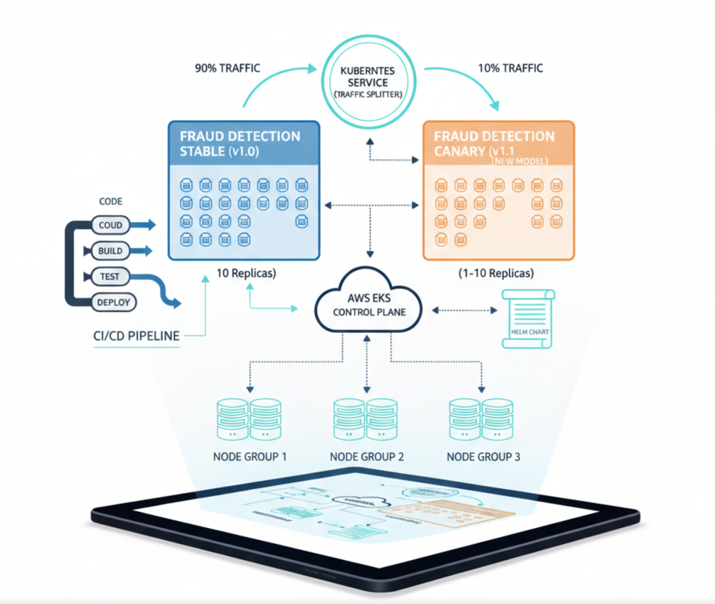
I deployed a managed Kubernetes cluster on AWS EKS with three node groups. The fraud detection service ran as a deployment with 10 replicas for stable production traffic. For canary deployments, I created a second deployment with 1–10 replicas representing the new model version. A Kubernetes service distributed traffic across both deployments proportionally based on replica count. I used Helm charts for consistent deployment configuration and integrated with the CI/CD pipeline for automated deployments.
Canary Deployment with Kubernetes
I configured Kubernetes to support gradual traffic shifting with label-based routing:
apiVersion: apps/v1
kind: Deployment
metadata:
  name: fraud-api-stable
spec:
  replicas: 10
  selector:
    matchLabels:
      app: fraud-api
      version: stable
  template:
    metadata:
      labels:
        app: fraud-api
        version: stable
---
apiVersion: apps/v1
kind: Deployment
metadata:
  name: fraud-api-canary
spec:
  replicas: 1  # 10% traffic
  selector:
    matchLabels:
      app: fraud-api
      version: canary
  template:
    metadata:
      labels:
        app: fraud-api
        version: canary
I built a controller to automate traffic shifting:
from kubernetes import client, config

class CanaryController:
    def __init__(self):
        config.load_kube_config()
        self.apps_api = client.AppsV1Api()

    def scale_canary(self, replicas):
        self.apps_api.patch_namespaced_deployment_scale(
            name='fraud-api-canary',
            namespace='default',
            body={'spec': {'replicas': replicas}}
        )

    def gradual_rollout(self, stages=[1, 2, 5, 10]):
        for replicas in stages:
            print(f"Scaling to {replicas} canary replicas")
            self.scale_canary(replicas)
            time.sleep(1800)  # Wait 30 minutes

            if not self.validate_metrics():
                self.rollback()
                return False

        return True
Canary deployment progressed through 10%, 25%, 50%, and 100% traffic allocation over one week, with validation at each stage.
Automated Rollback
I implemented a monitoring service that triggers automatic rollback on metric violations:
from prometheus_api_client import PrometheusConnect

class RollbackController:
    def __init__(self):
        self.prom = PrometheusConnect(url="http://prometheus:9090")
        self.thresholds = {'fpr': 0.15, 'error_rate': 0.05}

    def monitor(self):
        while True:
            if self.should_rollback():
                self.execute_rollback()
                break
            time.sleep(60)

    def should_rollback(self):
        fpr = self.query_metric('fraud_fpr')
        if fpr and fpr > self.thresholds['fpr']:
            return True
        return False

    def query_metric(self, metric_name):
        result = self.prom.custom_query(metric_name)
        return float(result[0]['value'][1]) if result else None

    def execute_rollback(self):
        # Scale canary to 0, stable to 10
        canary_controller.scale_canary(0)
        alert_team("Automatic rollback executed")
This system successfully performed one automatic rollback during testing when a dependency issue caused latency spikes.
Phase 5: Continuous Retraining Pipeline (Weeks 7–8)
The final component was an automated pipeline for weekly model retraining using fresh production data.
Tool Selection: Apache Airflow
What is Apache Airflow:
Apache Airflow is an open-source workflow orchestration platform for programmatically authoring, scheduling, and monitoring data pipelines. It represents workflows as Directed Acyclic Graphs (DAGs) of tasks with dependencies. It provides a web UI for monitoring, retry logic, and integration with numerous data systems.
Why I chose Apache Airflow:
I needed orchestration for the weekly training pipeline with multiple dependent steps. I evaluated Airflow, Prefect, Kubeflow Pipelines, and AWS Step Functions. I selected Airflow because:
- Python-native: Define workflows as Python code with full programmatic control
- Rich operator library: Pre-built operators for common tasks (PostgreSQL, S3, MLflow)
- Dependency management: Explicit task dependencies with automatic retry and failure handling
- Scheduling flexibility: Cron-based scheduling with backfill capabilities
- Monitoring UI: Web interface shows pipeline execution history and task logs
- Mature ecosystem: Large community, extensive documentation, proven at scale
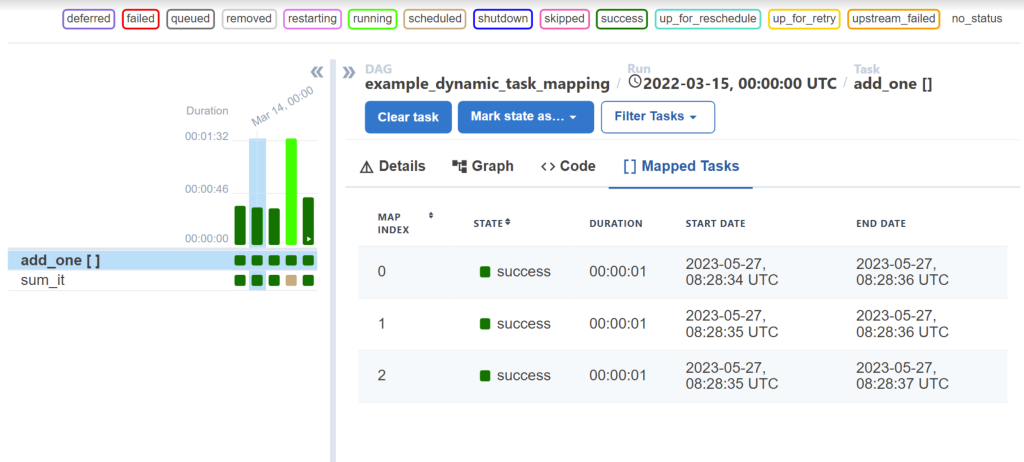
How I used it in this project:
I deployed Airflow on AWS EC2 with PostgreSQL as the metadata database. I created a DAG named “fraud_model_retraining” that executed every Monday at 2 AM. The DAG contained seven tasks: data validation, feature engineering, model training, evaluation, validation against production, registration in MLflow, and deployment to shadow mode. Each task had retry logic and sent failure notifications to Slack. The Airflow UI provided visibility into training pipeline execution and helped debug failures during initial implementation.
Training Pipeline Implementation with Airflow
from sklearn.model_selection import train_test_split
from xgboost import XGBClassifier
import mlflow

class TrainingPipeline:
    def __init__(self, db_connector):
        self.db = db_connector

    def fetch_training_data(self, days=90):
        query = """
            SELECT p.features, g.actual_label
            FROM predictions p
            JOIN ground_truth g ON p.transaction_id = g.transaction_id
            WHERE p.timestamp > NOW() - INTERVAL '%s days'
        """
        return pd.read_sql(query, self.db.conn, params=(days,))

    def train(self):
        df = self.fetch_training_data()

        if len(df) < 1000:
            raise ValueError("Insufficient training data")

        X = pd.json_normalize(df['features'])
        y = (df['actual_label'] == 'fraud').astype(int)

        X_train, X_test, y_train, y_test = train_test_split(
            X, y, test_size=0.2, stratify=y
        )

        with mlflow.start_run():
            model = XGBClassifier(
                max_depth=6,
                learning_rate=0.1,
                n_estimators=200,
                scale_pos_weight=(len(y_train) - y_train.sum()) / y_train.sum()
            )

            model.fit(X_train, y_train, eval_set=[(X_test, y_test)])

            metrics = self.evaluate(model, X_test, y_test)
            mlflow.log_metrics(metrics)
            mlflow.xgboost.log_model(model, "model")

            return mlflow.active_run().info.run_id, metrics

    def evaluate(self, model, X_test, y_test):
        from sklearn.metrics import precision_score, recall_score, f1_score

        y_pred = model.predict(X_test)

        return {
            'precision': precision_score(y_test, y_pred),
            'recall': recall_score(y_test, y_pred),
            'f1': f1_score(y_test, y_pred)
        }

    def validate(self, metrics, prod_metrics):
        if metrics['f1'] < prod_metrics['f1'] + 0.02:
            return False
        return True
Airflow DAG Configuration
I configured Apache Airflow to orchestrate weekly retraining:
from airflow import DAG
from airflow.operators.python import PythonOperator
from datetime import datetime, timedelta

dag = DAG(
    'fraud_model_retraining',
    schedule_interval='0 2 * * 1',  # Monday 2 AM
    start_date=datetime(2024, 1, 1),
    catchup=False
)

train_task = PythonOperator(
    task_id='train_model',
    python_callable=pipeline.train,
    dag=dag
)

validate_task = PythonOperator(
    task_id='validate_model',
    python_callable=pipeline.validate,
    dag=dag
)

deploy_task = PythonOperator(
    task_id='deploy_shadow',
    python_callable=deploy_to_shadow,
    dag=dag
)

train_task >> validate_task >> deploy_task
The pipeline executes automatically every Monday, trains on the latest labeled data, validates improvements, and deploys to shadow mode if validation passes.
Results and Impact

Financial Impact:
– Annual revenue recovery: $6.7M
– Infrastructure cost: $180K
– ROI: 3,722%
– Payback period: 11 days
Technical Stack Summary
- Monitoring: Prometheus, Grafana, Evidently AI, PagerDuty
- ML Infrastructure: MLflow, Apache Airflow
- Deployment: Kubernetes, Docker, Terraform
- Data: PostgreSQL, Kafka (future)
- Development: Python, XGBoost, scikit-learn, pandas
Key Technical Lessons
- Instrumentation is not optional
- Feedback loops create advantage
- Static thresholds fail in production
- Progressive deployment prevents failures
- Automation requires validation gates
- Business metrics matter more than ML metrics
Conclusion
The initial deployment failed because ML was treated as a one-time model deployment instead of an operational system.
The MLOps implementation transformed it into a continuously improving production service delivering measurable business value.
Eight weeks of engineering work turned a failing system into a multi-million-dollar impact platform.